Chapter 11 Chi-Square Tests
11.1 Description
Chi-square tests are a set of several non-parametric hypothesis tests used for categorical variables with nominal or ordinal measurement scale. There are three tests, the chi-square test of goodness of fit; the chi-square test of independence; and the chi-square test of homogeneity.
The goodness-of-fit test is used to determine whether sample data matches a given distribution.
The test of independence is used to determine whether there is a relationship between two categorical variables in a contingency table.
The test of homogeneity is used to determine whether two or more categorical variables with unknown distributions have the same distribution as each other in several populations.
11.2 Assumptions
Non-parametric tests and parametric tests make a number of assumptions that should hold true if the test is to be performed. Both types of testing assume the data was obtained through random selection, however it is not uncommon to find inferential statistics used when data has been collected from convenience samples and when this assumption is violated multiple replication studies will usually be performed to ensure confidence in the results.
The assumptions of the chi-square test are (McHugh M. L. 2013):
The data in the table must be counts or frequency data. It is not appropriate to use percentages or transformed data.
The categories of the variables should not overlap (e.g., male or female).
The chi-square test should not be used if the same subjects are tested at different time points.
The groups being compared must be independent and a different test should be used if they are related (e.g. paired samples).
The variables being compared must be categorised at the nominal level, although data that has been transformed from ordinal, interval or ratio data may also be used.
At least 80% of the cells should have expected values greater than or equal to five. Yates’s continuity correction can be used to to prevent overestimation of statistical significance when at least one entry has an expected count less than 5. Fisher’s exact test can also be used (Gonzalez-Chica D. A., Bastos J. L., Duquia R. P., Bonamigo R. R., Martínez-Mesa J. 2015).
No cell should have an expected value of zero.
11.3 Chi-Square Goodness of Fit (Distribution Test)
The chi-square Goodness-of-fit test, checks whether the frequencies of the individual characteristic values in the sample correspond to the frequencies of a defined distribution. In most cases, this defined distribution is that of the population.
In the general case the null and alternative hypotheses being tested are:
\(H_0\): The population fits the given distribution.
\(H_a\): The population does not fit the given distribution.
The chi-square value is calculated via:
\[\chi^2=\sum_{k=1}^{n}\frac{(O_k-E_k)^2}{E_k},\]
where \(O\) is the observed frequency and \(E\) is the expected frequency of the population.
The expected value is given by:
\[E=np_i,\] where \(n\) is the total sample size and \(p_i\) is the hypothesised population proportion of the i\(^{th}\) group.
The degrees of freedom also need to be calculated:
\[df=(p-1),\] where \(p\) is the number of categories.
A \(\chi^2\) table is used to compare the calculated value of \(\chi^2\) with critical values listed that correspond to the degrees of freedom and desired significance level.
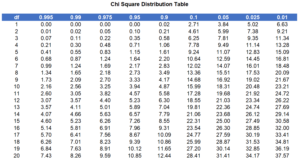
Table containing the critical values of the chi-square distribution.
You can also find these values using Excel with the function:
=CHISQ.INV.RT(p,df)
where p is the probability and df is the number of degrees of freedom.
11.3.1 Example
Rock-scissors-paper is a game of chance in which any player should be expected to win, tie and lose with equal frequency. Over the course of 30 games a player could be expected to win approximately ten times, lose ten times and tie times. Imagine a random sample of 24 games:
| Outcome | Frequency (Observed) |
|---|---|
| Win | 4 |
| Loss | 13 |
| Draw | 7 |
It does not seem like the outcomes occur with equal probability. It seems that the player is losing games much more frequently than games result in a draw or a win.
A \(\chi^2\) goodness of fit test could be used to determine if the distribution of these outcomes disagrees with an even distribution. This is essentially a hypothesis test:
\(H_0\): All the outcomes have equal probability.
\(H_a\): The outcomes do not have equal probability.
Since it is expected that the player should win, lose and draw with equal frequency the expected outcomes are 8 wins, 8 losses and 8 draws.
| Outcome | Frequency (Observed) | Frequency (Expected) |
|---|---|---|
| Win | 4 | 8 |
| Loss | 13 | 8 |
| Draw | 7 | 8 |
Calculating \(\chi^2\) gives:
\[\chi^2=\sum_{k=1}^{n}\frac{(O_k-E_k)^2}{E_k},\]
\[\chi^2=\frac{(4-8)^2}{8}+\frac{(13-8)^2}{8}+\frac{(7-8)^2}{8},\] \[\chi^2=\frac{(-4)^2}{8}+\frac{(5)^2}{8}+\frac{(-1)^2}{8},\] \[\chi^2=\frac{16}{8}+\frac{25}{8}+\frac{1}{8},\]
\[\chi^2=\frac{42}{8},\]
\[\chi^2=5.25.\]
After calculating \(\chi^2\) the number of degrees of freedom, df, is needed. This is given by:
\[df=(p-1),\]
where p is the number of categories.
There are three categories (win, lose or tie) so the degrees of freedom, df, is given by:
\[df=(3-1)=2.\] A \(\chi^2\) table is used to compare the calculated value of \(\chi^2\) with critical values that correspond to three degrees of freedom and a desired significance level.
For a \(df\) of 3 and a desired significance of 0.05 the calculated \(\chi^2\) value would need to be greater than 7.81 to reject the null hypothesis. In this case, \(\chi^2=5.25\) which is not greater than 7.81 so the null hypothesis is not rejected.
11.4 Chi-Square Test of Independence
The chi-square test of independence is used when two categorical variables are to be tested for independence.
In order to calculate the chi-square value, an observed and an expected frequency must be given. In the independence test, the expected frequency is the one that results when both variables are independent. If two variables are independent, the expected frequencies of the individual cells are obtained with:
\[\textrm{Expected Value}= \frac{\textrm{Row Total} \times \textrm{Column Total}}{\textrm{Grand Total}}.\] Note that this differs from the goodness of fit test.
The calculation of degrees of freedom also differs and is given by:
\[df=(p-1)(q-1),\]
where p is the number of rows and q is the number of columns.
11.5 Chi-Square Homogeneity Test
The chi-square homogeneity test can be used to check whether two or more samples come from the same population. The homogeneity and independence tests are performed in exactly the same way but there is a subtle difference.
| Test | Sample | Question |
|---|---|---|
| Independence | Two categorical variables are measured on one sample | Are the two categorical variables independent? |
| Homogeneity | A single categorical variable is measured on several samples | Are the groups homogeneous (have the same distribution of the categorical variable)? |
In practice these tests are performed identically and the difference lies in the question being asked and how results are reported.
11.6 Strength of Association
Different statistics can be used to calculate the effect size when a chi-squared test has been conducted, depending on the number of categories for each variable, the type of variables (nominal or ordinal) and the nature of the study.
11.6.1 Phi
In the case where there are only two categories for each variable, then effect size can be measured using phi (\(\phi\)). Phi is a measure for the strength of an association between two categorical variables in a 2 \(\times\) 2 contingency table. It is calculated by taking the chi-square value, dividing it by the sample size, and then taking the square root of this value (Akoglu, H. 2018).
This is calculated using the chi-square value (\(\chi^2\)) and the sample size (\(n\)), as follows:
\[\phi=\sqrt{\frac{\chi^2}{n}}.\]
In our case:
\[\phi=\sqrt{\frac{0.3125}{36}}=0.13.\]
This is considered a small effect (0.1 is considered a small effect size, 0.3 medium and 0.5 and above large).
Note also that an extension of ϕ for nominal variables with more than two categories is Cramer’s V, while other measures of effect size include relative risk and odds ratio.
11.6.2 Cramer’s V
Cramer’s V is an alternative to phi in tables bigger than 2 \(\times\) 2 tabules (Akoglu, H. 2018).
\[V = \sqrt{\frac{\chi^2}{n*\textrm{min}(r-1, c-1)}},\]
where \(n\) in the sample size and \(min()\) is the minimum of the two arguments \(r-1\) and \(c-1\). A Cramer’s V value of 0-0.29 indicates a weak association; 0.3-0.59 indicates a moderate association and a Cramer’s V of 0.6-1 indicates a strong association. The scale goes from complete independence to perfect association.
Association should never be greater than 1. A relatively weak correlation is all that can be expected when a phenomena is only partially dependent on the independent variable.
An alternative association measure for two nominal variables is the contingency coefficient. However, it’s better avoided since its maximum value depends on the dimensions of the contingency table involved.
For two ordinal variables, a Spearman correlation or Kendall’s tau are preferable over Cramér’s V. For two metric (interval or ratio) variables, a Pearson correlation is the preferred measure.
11.7 Example
This chi-square test could be useful in determining whether the duration of suspensions given to students in Northern Ireland differs by SEN status.
Data from the Education Authority, processed by the Department of Education for pupil suspensions across Northern Ireland for 2020/21 is presented below:
| Duration of Suspension | Non-SEN | SEN | Total | |
|---|---|---|---|---|
| 5 days | 2015 | 985 | 3000 | |
| 6 - 10 days | 152 | 165 | 317 | |
| 10 - 20 days | 64 | 74 | 138 | |
| 21+ days | 21 | 30 | 51 | |
| Total | 2252 | 1254 | 3506 |
Expected values are calculated using:
\[\textrm{Expected Value}= \frac{\textrm{Row Total} \times \textrm{Column Total}}{\textrm{Grand Total}}.\]
The results are shown below:
| Duration of Suspension | Non-SEN | SEN | Total | Non-SEN (expected) | SEN (expected) |
|---|---|---|---|---|---|
| 5 days | 2015 | 985 | 3000 | 1927 | 1073 |
| 6 - 10 days | 152 | 165 | 317 | 204 | 113 |
| 10 - 20 days | 64 | 74 | 138 | 89 | 50 |
| 21+ days | 21 | 30 | 51 | 33 | 18 |
| Total | 2252 | 1254 | 3506 | NA | NA |
Now calculate \(\chi^2\):
\[\chi^2=\frac{(1927-2015)^2}{2015} +\frac{(1073-985)^2}{985}+... + \frac{(18-30)^2}{30} = 78.8.\]
After calculating \(\chi^2\) the degrees of freedom, df, is needed to check the critical value on a look-up table. This is given by:
\[df=(p-1)(q-1)=(2-1)(4-1)=3.\]
For a significance level of 5% a \(\chi^2\) value greater than 3.84 is needed. Since the calculated \(\chi^2\) value is larger, there is a significant difference. The strength of the relationship can be determined using Cramer’s V. In this case, Cramer’s V is 0.15 which indicates a weak association. In practice, a Cramer’s V of 0.1, while weak, is usually sufficient to demonstrate that some association exists.
In 2020/21 there was a total of 1,254 compulsory school age pupils suspended who had SEN and 2,252 pupils who did not (NISRA 2022b). These numbers of pupils suspended represent 2.0% of pupils with SEN, and 0.9% for pupils with no SEN. While this does not provide any indication as to the possible links between duration of suspension and SEN status it does show that the rates of suspension are higher for pupils with SEN (NISRA 2022b).
In a real study more time would be spent determining the best way to record the data. For instance, Chi-square tests are sensitive to the bin width although most reasonable choices should produce similar results. It would also be possible to investigate frequency of suspension in terms of the number of times students were suspended rather than the duration of the suspension. It would also be useful to consider other factors such as whether students are eligible for free school meals, whether they are newcomers and break down the data by gender, ethnicity and the type of school attended. Inferential statistics are best used when substantial planning has been undertaken with regards to data collection. Ideally, a more complex logistic regression could be used to predict the odds of suspension for different genders based on a range of characteristic variables such as ethnicity, SEN status, FSM eligibility, etc.
11.8 Relative Risk
The relative risk (RR) and the odds ratio (OR) are widely used in medical research and are very commonly used measures of association in epidemiology (Schmidt C. O. and Kohlmann T. 2008). Relative risk is a comparison of the chance of an event happening in one group to the chance of it happening in another. For instance, the relative risk of lung cancer in smokers compared to non-smokers is the chance of getting lung cancer for smokers divided by the chance for non-smokers (Tenny S. and Hoffman M. R. 2022). Relative risk only shows the difference in likelihood between the two groups, it does not show the actual risk of the event happening (Tenny S. and Hoffman M. R. 2022).
The Relative Risk is used when comparing the probability of an event occurring to all possible events considered in a study.
For example consider the risk of developing cancer in those exposed and unexposed to second hand smoke. On a study’s conclusion we might have a table like the one below:
| Status | Disease | No Disease |
|---|---|---|
| Exposed | A | B |
| Unexposed | C | D |
To calculate the relative risk associated with an exposure we must compare the risk (incidence) among the exposed to those not exposed.
\[\textrm{Ratio of Risks} = \frac{\textrm{Disease Risk (incidence) in exposed (A/(A+B))}}{ \textrm{Disease Risk (incidence) in Non-Exposed (C/(C+D))}} = \textrm{Relative Risk}. \]
Let’s add values to do the calculations:
| Status | Disease | No Disease |
|---|---|---|
| Exposed | A | B |
| Unexposed | C | D |
\[\textrm{Disease Risk (incidence) in exposed}=\frac{366}{366+32}=0.92,\] \[\textrm{Disease Risk (incidence) in unexposed}=\frac{64}{64+319}=0.17,\]
\[\textrm{Relative Risk}=\frac{0.92}{0.17}=5.41.\] RR = 1 indicates that the incidence in the exposed is the same as the incidence in the non-exposed. No increased risk, no association.
RR > 1 indicates that the incidence in the exposed is greater than the incidence in the non-exposed. Increased risk, positive association.
RR < 1 indicates that the incidence in the exposed is lower than the incidence in the non exposed. Decreased risk, negative association.
The further the RR is from 1 the stronger the association.
The relative risk will be reported alongside a p value or a 95% confidence interval. If the p value is not less than 0.05 or if the confidence interval includes 1 then the RR is not statistically significant.
Information
You cannot calculate relative risk in a case control study. For instance, a study might involve a control group of 100 people without cancer and a group of 100 people with cancer. The disease rate might be 50% because of how the study was designed.
11.9 Odds Ratio
The odds ratio is used in cohort or case-control studies.
Information
Odds ratios consistently overestimate risk.
Odds are not the same as probability:
\[\textrm{Odds}=\frac{\textrm{Probability}}{1-\textrm{Probability}}.\]
For instance, a 60% probability to win gives 1.5 odds to win.
Given some data:
| Status | Disease (case) | Disease (Control |
|---|---|---|
| Exposed | A | B |
| Unexposed | C | D |
The Odds ratio is given by:
\[\textrm{Odds Ratio} = \frac{\textrm{odds that a case was exposed (A/C)}}{\textrm{odds that a control was exposed (B/D)}}.\]
Here’s an example with real data:
| Exposure: Parental smoking in pregnancy | Disease (Cancer) | No Disease (No Cancer) |
|---|---|---|
| Yes: Smoking | 87 | 147 |
| No: Non-Smoking | 201 | 508 |
The odds ratio is:
\[OR=\frac{(\frac{87}{201})}{(\frac{147}{508})}=1.48.\] This is different from the relative risk equation.
OR = 1 indicates that exposure is not associated with the disease.
OR > 1 indicates that exposure is positively associated with the disease.
OR < 1 indicates that exposure is negatively associated with the disease.
The further the OR is from 1, the stronger the association.
Summary
Goodness-of-fit
Use the goodness-of-fit test to decide whether a population with an unknown distribution “fits” a known distribution.
\(H_0\): The population fits the given distribution.
\(H_a\): The population does not fit the given distribution.
Independence
Use the test for independence to decide whether two variables (factors) are independent or dependent.
\(H_0\): The two variables (factors) are independent.
\(H_a\): The two variables (factors) are dependent.
Homogeneity
Use the test for homogeneity to decide if two or more populations with unknown distributions have the same distribution as each other.
\(H_0\): The two populations follow the same distribution.
\(H_a\): The two populations have different distributions.